Introduction to Splines

---

This is the second post in a multiple part series. The first post was on interpolation between two values. Here we will look at interpolation between multiple values.

Splines are mathematical functions to interpolate between several values. They are defined as piecewise polynomials, meaning that each interval is handled separately.

So, let's get started. For example, we will interpolate with 10 control points. The interpolation function will loop, so we also copy the first point to the end. Also note that these control points are uniformly spaced (at 0, .1, .2, .3, etc) on the X axis. In general we will try to avoid having uniform spacing as an absolute requirement because it's not always practical.

Our goal with a spline is to take in a list of inputs, Xs, and outputs, Ys, and produce a reasonable output for any given input. Each XY pair is called a control point, knot, or duck. The input into a spline function is usually labeled , for time.

Remember that splines are defined piecewise; a separate function can be written for each interval. The simplest spline uses the Step function for each interval. That is, it just jumps to the nearest control point. This is rarely useful, and mostly makes its way into programs by accident.

Next, we can use linear interpolation for each interval. Note that linear interpolation only considers the two surrounding control points for each interval. Because of this, it is very local. Any one control point only affects the interval immediately before and after it. We will also look at this spline's derivative. You can easily see that it's not continuous. If you prefer to think of the spline function as defining an object's position, then the derivative can be thought of as the object's speed. It not hard to imagine that linear interpolation gives a jerky appearance in animations, because of it's non-continuous speed and infinite acceleration.

Cosine interpolation fixes the non-continuous derivative, but introduces other problems. It forces the derivative at each control point to be 0. So, if cosine interpolation is used in animation, an object will slow down and stop at each control point. This is usually undesirable, but it can nevertheless sometimes be useful. Cosine interpolation is still local, it only every considers the immediately adjacent control points for each interval.

Cubic Hermite Splines

To get smoother interpolation it is desirable to consider more than just two control points for each interval. Natural cubic splines have global control, and the function always considers each control point. Catmull-Rom, Cardinal, and Kochanek-Bartels splines use four control points for each interval (that is the two immediately surrounding control points, and an extra control point on each side, for each interval). These last three splines are all types of cubic Hermite splines.

A cubic Hermite spline is a spline with each polynomial in Hermite form. Basically, each interval will use two control points and two tangents. These tangent values can be defined by the user, or defined automatically by more surrounding control points. First off, we need to define the four Hermite basis functions.

Each interval uses the four basis functions like so:

where and are the tangent values.

You can see that and scale the control points, while and scale the specified tangents. You can also quickly see that the spline will pass through each control point by considering the scaling factors from the graph above.

The tangents can be specified individually by an artist, or generated automatically. They are usually generated automatically, but to get a feel for the cubic Hermite spline I'll show an example where every tangent has been specified as 1. You can see that the function always has a slope of 1 at each control point. In other words, it passes through each control point at 45 degrees because that was the tangent specified.

Cardinal Splines

Given the control points , , , and we can use a Cardinal spline to interpolate between and .

Assuming uniformly spaced control points, a Cardinal spline defines the tangents as:

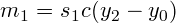
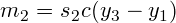
Where is a tension parameter. The tension parameter can intuitively be thought of as the length of the tangents. is a scaling factor for non-uniform control point spacing. If the control points are uniformly space, it can be omitted or set to 1. We'll cover non-uniform control point spacing below.

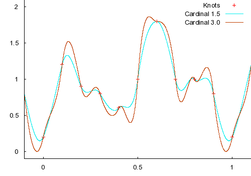
Here are some examples of Cardinal splines with various (tension) values:

It's straight forward to adapt the Cardinal spline for non-uniform control. However, it seems to be little known. A search online doesn't turn up much help and indeed a few sources even say it's non-trivial or even impossible (due to the curvature of the curves, uh-huh). That's not true. Using non-uniformly spaced control points is actually quite straightforward.

For non-uniform control points, each tangent simply needs scaled. First we'll define a few variables useful for the control point spacing.

Then the scaling factors are:

Non-uniform control point spacing is incredibly useful for animation key-framing. With uniform control points an artist would have to specify the models' positions every fixed amount of time (e.g. every half second). With non-uniform control point spacing, an animation artist can specify models' positions whenever convenient.

Catmull-Rom Splines

A Cardinal spline with a tension of .5 is a special case. It's then called a Catmull-Rom spline. Catmull-Rom splines are thought to be esthetically pleasing and are quite common.

Two Dimensional Splines

Wrapping up, we'll take a quick look at two dimensional splines. It should first be noted that the X and Y axis can be interpolated completely separate. This makes sense since the axises are orthogonal, and a movement on one axis does not affect the other axis at all. Good spline code should be written generically and work equally well with a single number or a vector. In C++ this is easily accomplished with templates, which allows the same code to be used for one or more dimensions.

Next up we'll look at arc-length parametrization.

---

---